三天速成！香港科技大學TensorFlow課件分享

原標題：三天速成！香港科技大學TensorFlow課件分享

機器之心整理

參與：蔣思源

這是一套香港科技大學發佈的極簡 TensorFlow 入門教程，三天全套幻燈片教程已被分享到 Google Drive。機器之心將簡要介紹該教程並藉此梳理 TensorFlow 的入門概念與實現。

該教程第一天先介紹了深度學習和機器學習的潛力與基本概念，而後便開始探討深度學習框架 TensorFlow。首先我們將學到如何安裝 TensorFlow，其實我們感覺 TensorFlow 環境配置還是相當便捷的，基本上按照官網的教程就能完成安裝。隨後就從「Hello TensorFlow」開始依次講解計算圖、佔位符、張量等基本概念。

當然我們真正地理解 TensorFlow 還需要從實戰出發一點點學習那些最基本的概念，因此第一天重點講解了線性迴歸、Logistic 迴歸、Softmax 分類和神經網絡。每一個模型都從最基本的概念出發先推導運行過程，然後再結合 TensorFlow 講解張量、計算圖等真正的意義。神經網絡這一部分講解得十分詳細，我們將從最基本的感知機原理開始進而使用多層感知機解決異或問題（XOR），重點是該課程詳細推導了前向傳播與反向傳播的數學過程並配以 TensorFlow 實現。

教程第二天詳細地討論了卷積神經網絡，它從 TensorFlow 的訓練與構建技巧開始，解釋了應用於神經網絡的各種權重初始化方法、激活函數、損失函數、正則化和各種優化方法等。在教程隨後論述 CNN 原理的部分，我們可以看到大多是根據斯坦福 CS231n 課程來解釋的。第二天最後一部分就是使用 TensorFlow 實現前面的理論，該教程使用單獨的代碼塊解釋了 CNN 各個部分的概念，比如說 2 維卷積層和最大池化層等。

教程第三天詳解了循環神經網絡，其從時序數據開始先講解了 RNN 的基本概念與原理，包括編碼器-解碼器模式、注意力機制和門控循環單元等非常先進與高效的機制。該教程後一部分使用了大量的實現代碼來解釋前面我們所瞭解的循環神經網絡基本概念，包括 TensorFlow 中單個循環單元的構建、批量輸入與循環層的構建、RNN 序列損失函數的構建、訓練計算圖等。

下面機器之心將根據該教程資料簡要介紹 TensorFlow 基本概念和 TensorFlow 機器學習入門實現。更詳細的內容請查看香港科技大學三日 TensorFlow 速成課程資料

• 三日速成課程 Google Drive 資料地址：https://drive.google.com/drive/folders/0B41Zbb4c8HVyY1F5Ml94Z2hodkE

• 三日速成課程百度雲盤資料地址：http://pan.baidu.com/s/1boGGzeR

TensorFlow 基礎

本小節將從張量與圖、常數與變量還有佔位符等基本概念出發簡要介紹 TensorFlow。需要進一步瞭解 TensorFlow 的讀者可以閱讀谷歌 TensorFlow 的文檔，當然也可以閱讀其他中文教程或書籍，例如《TensorFlow：實戰 Google 深度學習框架》和《TensorFlow 實戰》等。

• TensorFlow 文檔地址：https://www.tensorflow.org/get_started/

1. 圖

TensorFlow 是一種採用數據流圖（data flow graphs），用於數值計算的開源軟件庫。其中 Tensor 代表傳遞的數據爲張量（多維數組），Flow 代表使用計算圖進行運算。數據流圖用「結點」（nodes）和「邊」（edges）組成的有向圖來描述數學運算。「結點」一般用來表示施加的數學操作，但也可以表示數據輸入的起點和輸出的終點，或者是讀取/寫入持久變量（persistent variable）的終點。邊表示結點之間的輸入/輸出關係。這些數據邊可以傳送維度可動態調整的多維數據數組，即張量（tensor）。

在 Tensorflow 中，所有不同的變量和運算都是儲存在計算圖。所以在我們構建完模型所需要的圖之後，還需要打開一個會話（Session）來運行整個計算圖。在會話中，我們可以將所有計算分配到可用的 CPU 和 GPU 資源中。

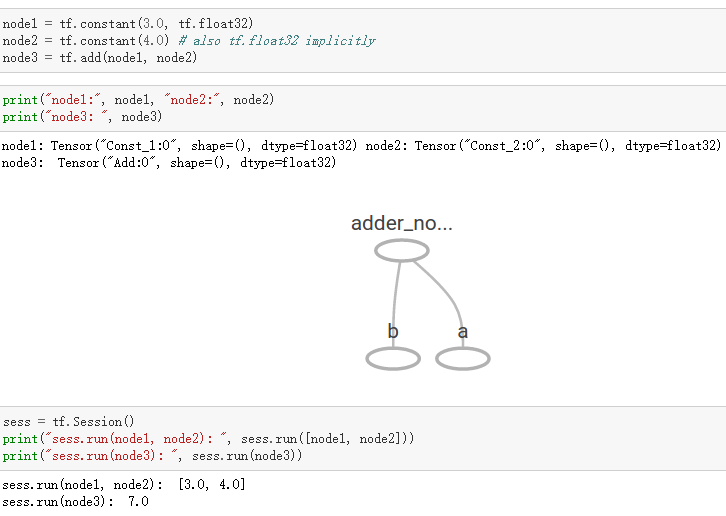
如上所示我們構建了一個加法運算的計算圖，第二個代碼塊並不會輸出計算結果，因爲我們只是定義了一張圖，而沒有運行它。第三個代碼塊纔會輸出計算結果，因爲我們需要創建一個會話（Session）才能管理 TensorFlow 運行時的所有資源。但計算完畢後需要關閉會話來幫助系統回收資源，不然就會出現資源泄漏的問題。

TensorFlow 中最基本的單位是常量（Constant）、變量（Variable）和佔位符（Placeholder）。常量定義後值和維度不可變，變量定義後值可變而維度不可變。在神經網絡中，變量一般可作爲儲存權重和其他信息的矩陣，而常量可作爲儲存超參數或其他結構信息的變量。在上面的計算圖中，結點 1 和結點 2 都是定義的常量 tf.constant()。我們可以分別聲明不同的常量（tf.constant()）和變量（tf.Variable()），其中 tf.float 和 tf.int 分別聲明瞭不同的浮點型和整數型數據。

2. 佔位符和 feed_dict

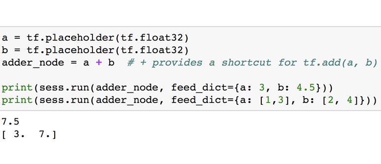
TensorFlow 同樣還支持佔位符，佔位符並沒有初始值，它只會分配必要的內存。在會話中，佔位符可以使用 feed_dict 饋送數據。

feed_dict 是一個字典，在字典中需要給出每一個用到的佔位符的取值。在訓練神經網絡時需要每次提供一個批量的訓練樣本，如果每次迭代選取的數據要通過常量表示，那麼 TensorFlow 的計算圖會非常大。因爲每增加一個常量，TensorFlow 都會在計算圖中增加一個結點。所以說擁有幾百萬次迭代的神經網絡會擁有極其龐大的計算圖，而佔位符卻可以解決這一點，它只會擁有佔位符這一個結點。

3. 張量

在 TensorFlow 中，張量是計算圖執行運算的基本載體，我們需要計算的數據都以張量的形式儲存或聲明。如下所示，該教程給出了各階張量的意義。

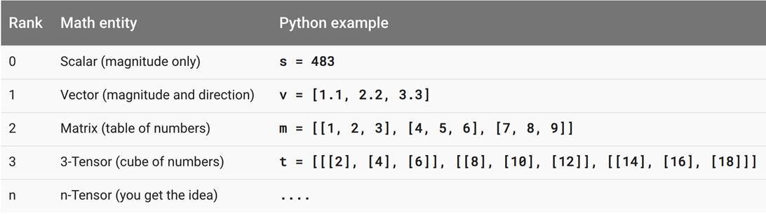
零階張量就是我們熟悉的標量數字，它僅僅只表達了量的大小或性質而沒有其它的描述。一階張量即我們熟悉的向量，它不僅表達了線段量的大小，同時還表達了方向。一般來說二維向量可以表示平面中線段的量和方向，三維向量和表示空間中線段的量和方向。二階張量即矩陣，我們可以看作是填滿數字的一個表格，矩陣運算即一個表格和另外一個表格進行運算。當然理論上我們可以產生任意階的張量，但在實際的機器學習算法運算中，我們使用得最多的還是一階張量（向量）和二階張量（矩陣）。

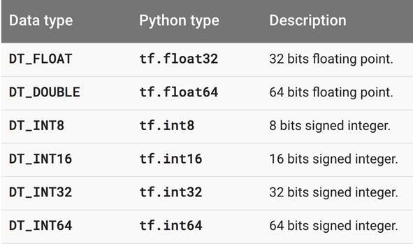
一般來說，張量中每個元素的數據類型有以上幾種，即浮點型和整數型，一般在神經網絡中比較常用的是 32 位浮點型。

4. TensorFlow 機器

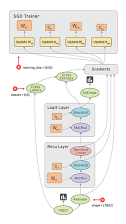
在整個教程中，下面一張示意圖將反覆出現，這基本上是所有 TensorFlow 機器學習模型所遵循的構建流程，即構建計算圖、饋送輸入張量、更新權重並返回輸出值。

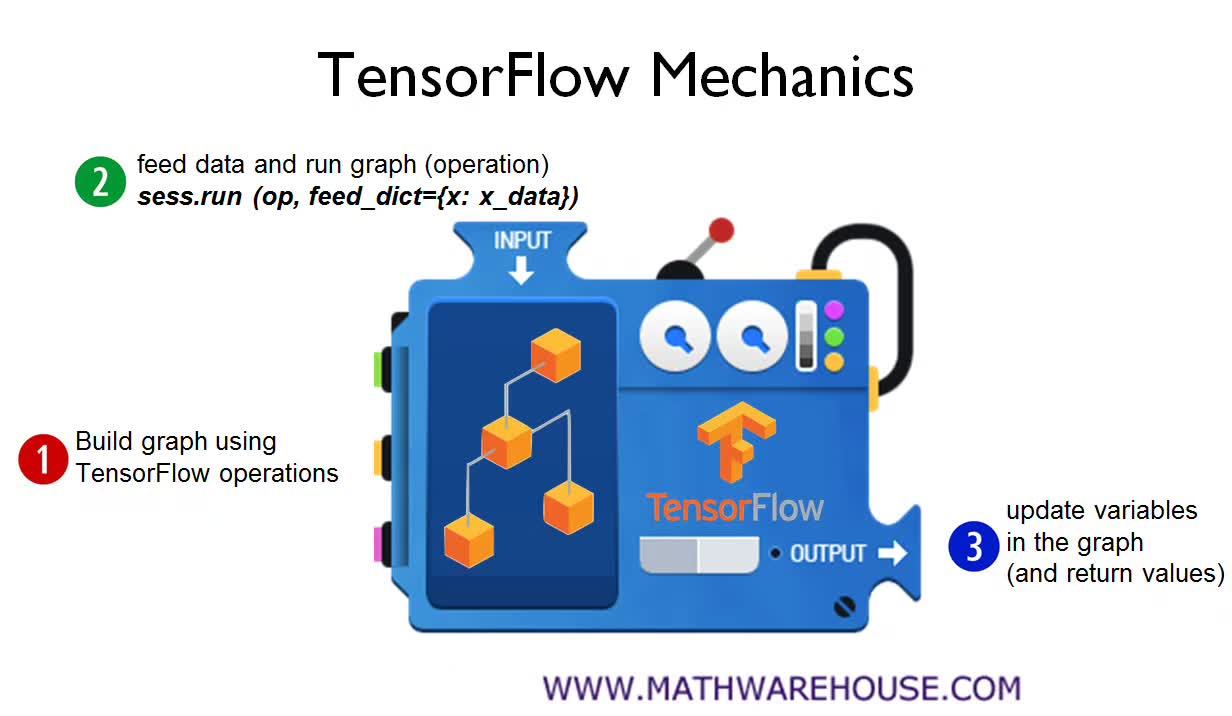
在第一步使用 TensorFlow 構建計算圖中，我們需要構建整個模型的架構。例如在神經網絡模型中，我們需要從輸入層開始構建整個神經網絡的架構，包括隱藏層的數量、每一層神經元的數量、層級之間連接的情況與權重、整個網絡每個神經元使用的激活函數等內容。此外，我們還需要配置整個訓練、驗證與測試的過程。例如在神經網絡中，定義整個正向傳播的過程與參數並設定學習率、正則化率和批量大小等各類訓練超參數。第二步需要將訓練數據或測試數據等饋送到模型中，TensorFlow 在這一步中一般需要打開一個會話（Session）來執行參數初始化和饋送數據等任務。例如在計算機視覺中，我們需要隨機初始化整個模型參數數值，並將圖像成批（圖像數等於批量大小）地饋送到定義好的卷積神經網絡中。第三步即更新權重並獲取返回值，這個一般是控制訓練過程與獲得最終的預測結果。

TensorFlow 模型實戰TensorFlow 線性迴歸

該教程前面介紹了很多線性迴歸的基本概念，包括直線擬合、損失函數、梯度下降等基礎內容。我們一直認爲線性迴歸是理解機器學習最好的入門模型，因爲他的原理和概念十分簡單，但又基本涉及到了機器學習的各個過程。總的來說，線性迴歸模型可以用下圖概括：

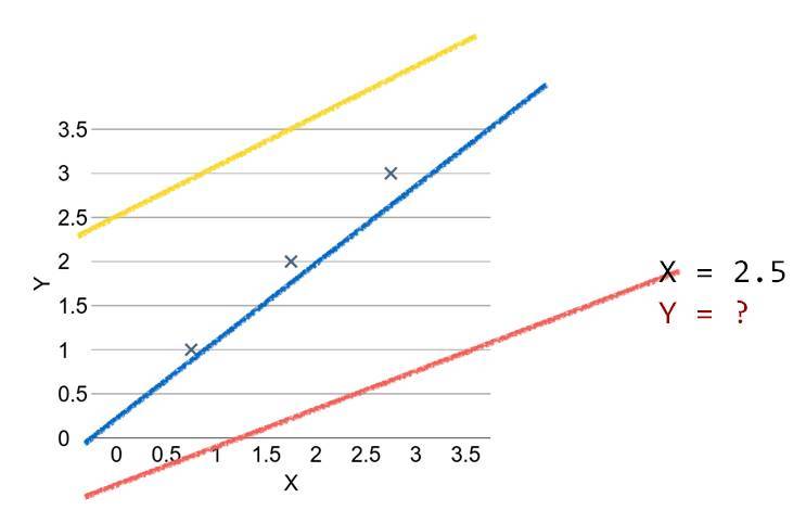
其中「×」爲數據點，我們需要找到一條直線以最好地擬合這些數據點。該直線和這些數據點之間的距離即損失函數，所以我們希望找到一條能令損失函數最小的直線。以下是使用 TensorFlow 構建線性迴歸的簡單案例。

1. 構建目標函數（即「直線」）

目標函數即 H(x)=Wx+b，其中 x 爲特徵向量、W 爲特徵向量中每個元素對應的權重、b 爲偏置項。

1. #X and Y data

2. x_train =[1,2,3]

3. y_train =[1,2,3]

6. W =tf.Variable(tf.random_normal([1]),name='weight')

7. b =tf.Variable(tf.random_normal([1]),name='bias')

8. #Ourhypothesis XW+b

9. hypothesis =x_train *W +b

如上所示，我們定義了 y=wx+b 的運算，即我們需要擬合的一條直線。

2. 構建損失函數

下面我們需要構建整個模型的損失函數，即各數據點到該直線的距離，這裏我們構建的損失函數爲均方誤差函數：

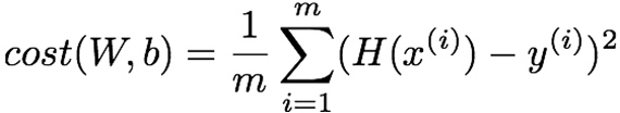
該函數表明根據數據點預測的值和該數據點真實值之間的距離，我們可以使用以下代碼實現：

1. #cost/loss function

2. cost =tf.reduce_mean(tf.square(hypothesis -y_train))

其中 tf.square() 爲取某個數的平方，而 tf.reduce_mean() 爲取均值。

3. 採用梯度下降更新權重

1. #Minimize

2. optimizer =tf.train.GradientDescentOptimizer(learning_rate=0.01)

3. train =optimizer.minimize(cost)

爲了尋找能擬合數據的最好直線，我們需要最小化損失函數，即數據與直線之間的距離，因此我們可以採用梯度下降算法：

4. 運行計算圖執行訓練

1. #Launchthe graph in a session.

2. sess =tf.Session()

3. #Initializesglobal variables in the graph.

4. sess.run(tf.global_variables_initializer())

6. #Fitthe line

7. forstep in range(2001):

8. sess.run(train)

9. ifstep %20==0:

10. print(step,sess.run(cost),sess.run(W),sess.run(b))

上面的代碼打開了一個會話並執行變量初始化和饋送數據。

最後，該課程給出了完整的實現代碼，剛入門的讀者可以嘗試實現這一簡單的線性迴歸模型：

1. importtensorflow as tf

2. W =tf.Variable(tf.random_normal([1]),name='weight')

3. b =tf.Variable(tf.random_normal([1]),name='bias')

5. X =tf.placeholder(tf.float32,shape=[None])

6. Y =tf.placeholder(tf.float32,shape=[None])

8. #Ourhypothesis XW+b

9. hypothesis =X *W +b

10. #cost/loss function

11. cost =tf.reduce_mean(tf.square(hypothesis -Y))

12. #Minimize

13. optimizer =tf.train.GradientDescentOptimizer(learning_rate=0.01)

14. train =optimizer.minimize(cost)

16. #Launchthe graph in a session.

17. sess =tf.Session()

18. #Initializesglobal variables in the graph.

19. sess.run(tf.global_variables_initializer())

21. #Fitthe line

22. forstep in range(2001):

23. cost_val,W_val,b_val,_ =sess.run([cost,W,b,train],

24. feed_dict={X:[1,2,3],Y:[1,2,3]})

25. ifstep %20==0:

26. print(step,cost_val,W_val,b_val)

下面讓我們概覽該課程更多的內容。

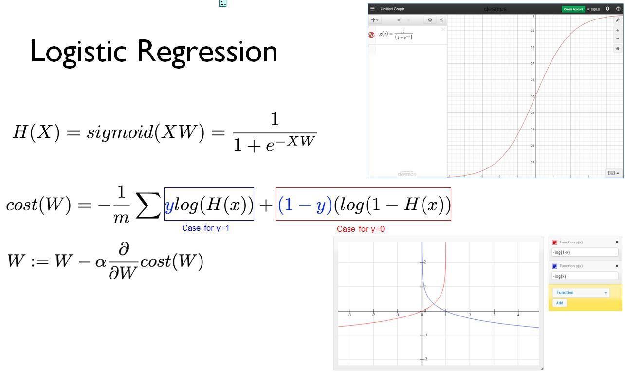
Logistic 迴歸

該課程照例先簡介了 Logistic 迴歸的基本概念，如下展示了目標函數、損失函數和權重更新過程。

後面展示了 Logistic 迴歸的實現代碼：

1. xy =np.loadtxt('data-03-diabetes.csv',delimiter=',',dtype=np.float32)

2. x_data =xy[:,0:-1]

3. y_data =xy[:,[-1]]

5. #placeholders fora tensor that will be always fed.

6. X =tf.placeholder(tf.float32,shape=[None,8])

7. Y =tf.placeholder(tf.float32,shape=[None,1])

9. W =tf.Variable(tf.random_normal([8,1]),name='weight')

10. b =tf.Variable(tf.random_normal([1]),name='bias')

12. #Hypothesisusing sigmoid:tf.div(1.,1.+tf.exp(tf.matmul(X,W)))

13. hypothesis =tf.sigmoid(tf.matmul(X,W)+b)

14. #cost/loss function

15. cost =-tf.reduce_mean(Y *tf.log(hypothesis)+(1-Y)*tf.log(1-hypothesis))

16. train =tf.train.GradientDescentOptimizer(learning_rate=0.01).minimize(cost)

18. #Accuracycomputation

19. #Trueifhypothesis>0.5elseFalse

20. predicted =tf.cast(hypothesis >0.5,dtype=tf.float32)

21. accuracy =tf.reduce_mean(tf.cast(tf.equal(predicted,Y),dtype=tf.float32))

23. #Launchgraph

24. withtf.Session()as sess:

25. sess.run(tf.global_variables_initializer())

27. feed ={X:x_data,Y:y_data}

28. forstep in range(10001):

29. sess.run(train,feed_dict=feed)

30. ifstep %200==0:

31. print(step,sess.run(cost,feed_dict=feed))

33. #Accuracyreport

34. h,c,a =sess.run([hypothesis,predicted,accuracy],feed_dict=feed)

35. print("nHypothesis: ",h,"nCorrect (Y): ",c,"nAccuracy: ",a)

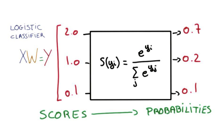
Softmax 分類

下圖展示了 Softmax 的基本方法，它可以產生和爲 1 的類別概率。

以下代碼爲 Softmax 分類器處理 MNIST 數據集：

1. #weights &bias fornn layers

2. W =tf.Variable(tf.random_normal([784,10]))

3. b =tf.Variable(tf.random_normal([10]))

4. hypothesis =tf.matmul(X,W)+b

5. #define cost/loss &optimizer

6. cost =tf.reduce_mean(tf.nn.softmax_cross_entropy_with_logits(logits=hypothesis,labels=Y))

7. optimizer =tf.train.AdamOptimizer(learning_rate=learning_rate).minimize(cost)

8. #initialize

9. sess =tf.Session()

10. sess.run(tf.global_variables_initializer())

12. #train my model

13. forepoch in range(training_epochs):

14. avg_cost =0

15. total_batch =int(mnist.train.num_examples /batch_size)

17. fori in range(total_batch):

18. batch_xs,batch_ys =mnist.train.next_batch(batch_size)

19. feed_dict ={X:batch_xs,Y:batch_ys}

20. c,_ =sess.run([cost,optimizer],feed_dict=feed_dict)

21. avg_cost +=c /total_batch

23. print('Epoch:','%04d'%(epoch +1),'cost =','{:.9f}'.format(avg_cost))

25. print('Learning Finished!')

27. #Testmodel and check accuracy

28. correct_prediction =tf.equal(tf.argmax(hypothesis,1),tf.argmax(Y,1))

29. accuracy =tf.reduce_mean(tf.cast(correct_prediction,tf.float32))

30. print('Accuracy:',sess.run(accuracy,feed_dict={X:mnist.test.images,Y:mnist.test.labels}))

神經網絡

下圖簡要介紹了神經網絡的運算過程，這一部分十分詳細，對於初學者來說是難得的資料：

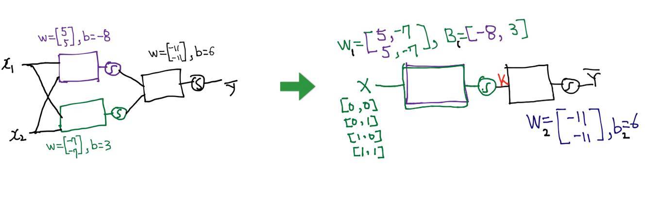
下面是該教程採用神經網絡解決異或問題的代碼，異或問題是十分經典的任務，我們可以從該問題中理解神經網絡的強大之處：

1. x_data =np.array([[0,0],[0,1],[1,0],[1,1]],dtype=np.float32)

2. y_data =np.array([[0],[1],[1],[0]],dtype=np.float32)

3. X =tf.placeholder(tf.float32)

4. Y =tf.placeholder(tf.float32)

6. W1 =tf.Variable(tf.random_normal([2,2]),name='weight1')

7. b1 =tf.Variable(tf.random_normal([2]),name='bias1')

8. layer1 =tf.sigmoid(tf.matmul(X,W1)+b1)

10. W2 =tf.Variable(tf.random_normal([2,1]),name='weight2')

11. b2 =tf.Variable(tf.random_normal([1]),name='bias2')

12. hypothesis =tf.sigmoid(tf.matmul(layer1,W2)+b2)

14. #cost/loss function

15. cost =-tf.reduce_mean(Y *tf.log(hypothesis)+(1-Y)*tf.log(1-hypothesis))

16. train =tf.train.GradientDescentOptimizer(learning_rate=0.1).minimize(cost)

17. #Accuracycomputation

18. #Trueifhypothesis>0.5elseFalse

19. predicted =tf.cast(hypothesis >0.5,dtype=tf.float32)

20. accuracy =tf.reduce_mean(tf.cast(tf.equal(predicted,Y),dtype=tf.float32))

21. #Launchgraph

22. withtf.Session()as sess:

23. #InitializeTensorFlowvariables

24. sess.run(tf.global_variables_initializer())

25. forstep in range(10001):

26. sess.run(train,feed_dict={X:x_data,Y:y_data})

27. ifstep %100==0:

28. print(step,sess.run(cost,feed_dict={X:x_data,Y:y_data}),sess.run([W1,W2]))

30. #Accuracyreport

31. h,c,a =sess.run([hypothesis,predicted,accuracy],

32. feed_dict={X:x_data,Y:y_data})

33. print("nHypothesis: ",h,"nCorrect: ",c,"nAccuracy: ",a)

卷積神經網絡

第二天教程就正式進入卷積神經網絡，我們只能用下圖展示卷積神經網絡大概的架構，更多資料請查看原課程課件：

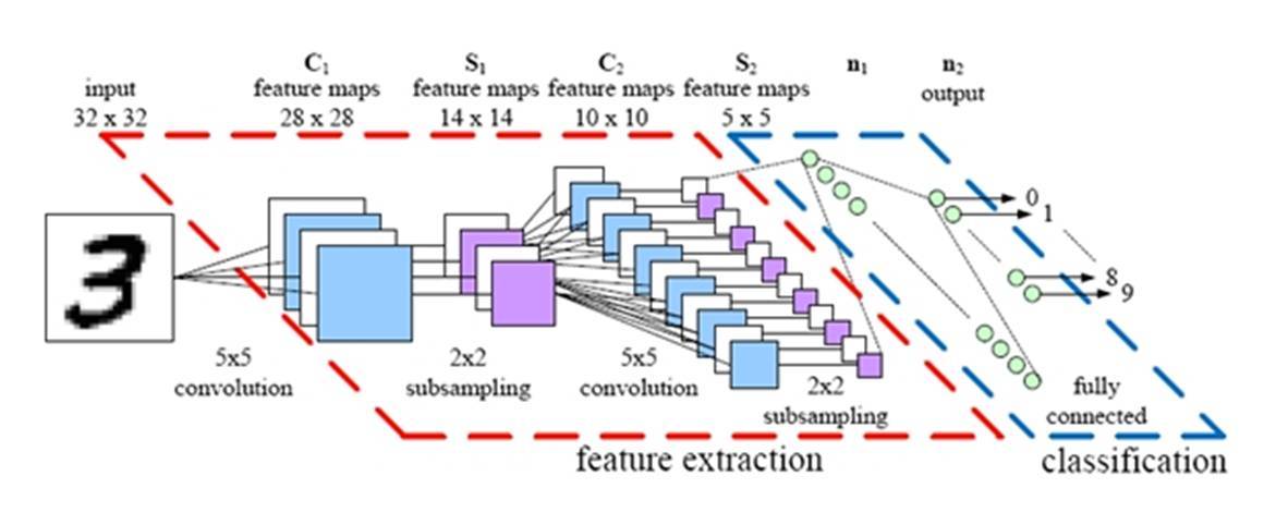
該教程同樣提供了很多卷積網絡的實現代碼，下面我們簡要介紹一個簡單的卷積神經網絡實現過程，該卷積神經網絡的架構如下：

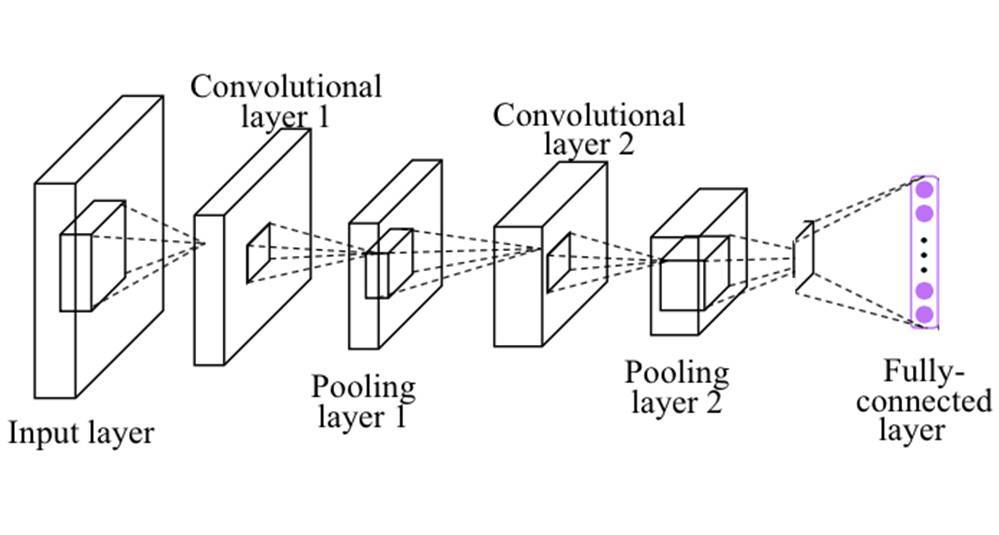
下面的代碼穿件了第一個卷積層，即上圖卷積層 1 和池化層 1：

1. #input placeholders

2. X =tf.placeholder(tf.float32,[None,784])

3. X_img =tf.reshape(X,[-1,28,28,1])#img 28x28x1(black/white)

4. Y =tf.placeholder(tf.float32,[None,10])

6. #L1 ImgInshape=(?,28,28,1)

7. W1 =tf.Variable(tf.random_normal([3,3,1,32],stddev=0.01))

8. #Conv->(?,28,28,32)

9. #Pool->(?,14,14,32)

10. L1 =tf.nn.conv2d(X_img,W1,strides=[1,1,1,1],padding='SAME')

11. L1 =tf.nn.relu(L1)

12. L1 =tf.nn.max_pool(L1,ksize=[1,2,2,1],

13. strides=[1,2,2,1],padding='SAME')

14. '''

15. Tensor("Conv2D:0",shape=(?,28,28,32),dtype=float32)

16. Tensor("Relu:0",shape=(?,28,28,32),dtype=float32)

17. Tensor("MaxPool:0",shape=(?,14,14,32),dtype=float32)

18. '''

後面的代碼構建了第二個卷積層，即上圖中的卷積層 2 和池化層 2：

1. '''

2. Tensor("Conv2D:0",shape=(?,28,28,32),dtype=float32)

3. Tensor("Relu:0",shape=(?,28,28,32),dtype=float32)

4. Tensor("MaxPool:0",shape=(?,14,14,32),dtype=float32)

5. '''

7. #L2 ImgInshape=(?,14,14,32)

8. W2 =tf.Variable(tf.random_normal([3,3,32,64],stddev=0.01))

9. #Conv->(?,14,14,64)

10. #Pool->(?,7,7,64)

11. L2 =tf.nn.conv2d(L1,W2,strides=[1,1,1,1],padding='SAME')

12. L2 =tf.nn.relu(L2)

13. L2 =tf.nn.max_pool(L2,ksize=[1,2,2,1],strides=[1,2,2,1],padding='SAME')

14. L2 =tf.reshape(L2,[-1,7*7*64])

15. '''

16. Tensor("Conv2D_1:0",shape=(?,14,14,64),dtype=float32)

17. Tensor("Relu_1:0",shape=(?,14,14,64),dtype=float32)

18. Tensor("MaxPool_1:0",shape=(?,7,7,64),dtype=float32)

19. Tensor("Reshape_1:0",shape=(?,3136),dtype=float32)

最後我們只需要構建一個全連接層就完成了整個 CNN 架構的搭建，即用以下代碼構建上圖最後紫色的全連接層：

1. '''

2. Tensor("Conv2D_1:0",shape=(?,14,14,64),dtype=float32)

3. Tensor("Relu_1:0",shape=(?,14,14,64),dtype=float32)

4. Tensor("MaxPool_1:0",shape=(?,7,7,64),dtype=float32)

5. Tensor("Reshape_1:0",shape=(?,3136),dtype=float32)

6. '''

7. L2 =tf.reshape(L2,[-1,7*7*64])

9. #FinalFC 7x7x64inputs ->10outputs

10. W3 =tf.get_variable("W3",shape=[7*7*64,10],initializer=tf.contrib.layers.xavier_initializer())

11. b =tf.Variable(tf.random_normal([10]))

12. hypothesis =tf.matmul(L2,W3)+b

14. #define cost/loss &optimizer

15. cost =tf.reduce_mean(tf.nn.softmax_cross_entropy_with_logits(logits=hypothesis,labels=Y))

16. optimizer =tf.train.AdamOptimizer(learning_rate=learning_rate).minimize(cost)

最後我們只需要訓練該 CNN 就完成了整個模型：

1. #initialize

2. sess =tf.Session()

3. sess.run(tf.global_variables_initializer())

5. #train my model

6. print('Learning stared. It takes sometime.')

7. forepoch in range(training_epochs):

8. avg_cost =0

9. total_batch =int(mnist.train.num_examples /batch_size)

10. fori in range(total_batch):

11. batch_xs,batch_ys =mnist.train.next_batch(batch_size)

12. feed_dict ={X:batch_xs,Y:batch_ys}

13. c,_,=sess.run([cost,optimizer],feed_dict=feed_dict)

14. avg_cost +=c /total_batch

15. print('Epoch:','%04d'%(epoch +1),'cost =','{:.9f}'.format(avg_cost))

17. print('Learning Finished!')

19. #Testmodel and check accuracy

20. correct_prediction =tf.equal(tf.argmax(hypothesis,1),tf.argmax(Y,1))

21. accuracy =tf.reduce_mean(tf.cast(correct_prediction,tf.float32))

22. print('Accuracy:',sess.run(accuracy,feed_dict={X:mnist.test.images,Y:mnist.test.labels}))

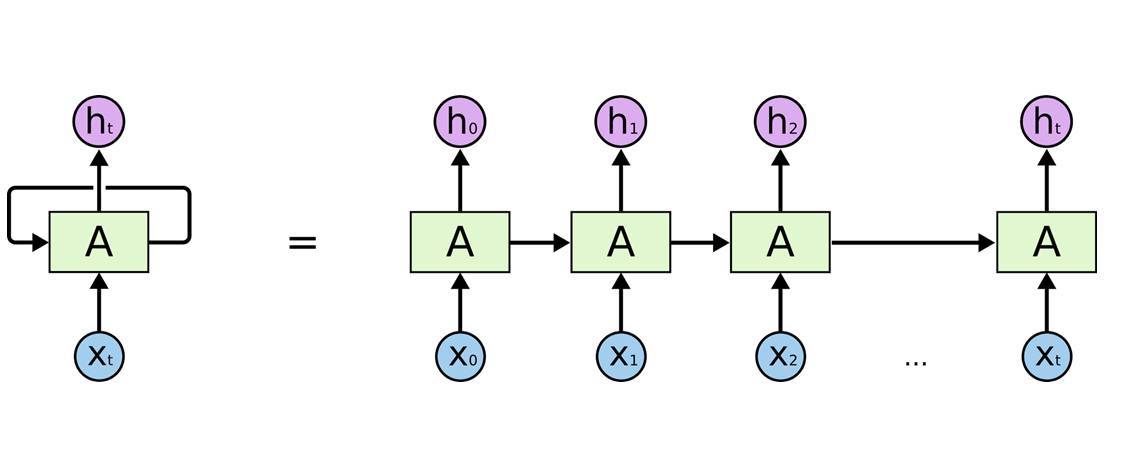
循環神經網絡

該教程第三天講述了循環神經網絡，下圖展示了循環單元的展開，循環單元是處理時序數據的核心。更詳細的資料請查看該課程課件。

以下 TensorFlow 代碼定義了簡單的循環單元：

1. #Onecell RNN input_dim (4)->output_dim (2)

2. hidden_size =2

3. cell =tf.contrib.rnn.BasicRNNCell(num_units=hidden_size)

5. x_data =np.array([[[1,0,0,0]]],dtype=np.float32)

6. outputs,_states =tf.nn.dynamic_rnn(cell,x_data,dtype=tf.float32)

8. sess.run(tf.global_variables_initializer())

9. pp.pprint(outputs.eval())

下面該課程展示了一個簡單的卷積神經網絡案例，如下所示，該案例訓練一個 RNN 以輸出「hihello」。

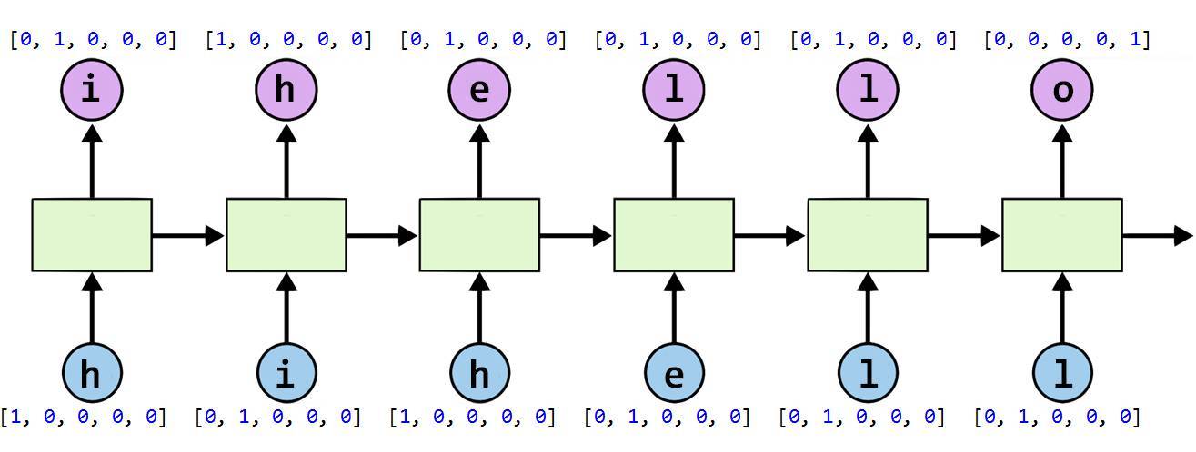
1. 創建 RNN 單元

如下可知 TensorFlow 中一般可以創建 3 種 RNN 單元，即 RNN 單元、LSTM 單元和 GRU 單元

# RNN modelrnn_cell = rnn_cell.BasicRNNCell(rnn_size)rnn_cell = rnn_cell. BasicLSTMCell(rnn_size)rnn_cell = rnn_cell. GRUCell(rnn_size)

2. 執行 RNN

# RNN modelrnn_cell = rnn_cell.BasicRNNCell(rnn_size)outputs, _states = tf.nn.dynamic_rnn( rnn_cell, X, initial_state=initial_state, dtype=tf.float32)

3. 設定 RNN 的參數

hidden_size = 5 # output from the LSTMinput_dim = 5 # one-hot sizebatch_size = 1 # one sentencesequence_length = 6 # |ihello| == 6

4. 創建數據

idx2char = ['h', 'i', 'e', 'l', 'o'] # h=0, i=1, e=2, l=3, o=4x_data = [[0, 1, 0, 2, 3, 3]] # hihellx_one_hot = [[[1, 0, 0, 0, 0], # h 0 [0, 1, 0, 0, 0], # i 1 [1, 0, 0, 0, 0], # h 0 [0, 0, 1, 0, 0], # e 2 [0, 0, 0, 1, 0], # l 3 [0, 0, 0, 1, 0]]] # l 3y_data = [[1, 0, 2, 3, 3, 4]] # ihelloX = tf.placeholder(tf.float32, [None, sequence_length, input_dim]) # X one-hotY = tf.placeholder(tf.int32, [None, sequence_length]) # Y label

5. 將數據饋送到 RNN 中

X = tf.placeholder( tf.float32, [None, sequence_length, hidden_size]) # X one-hotY = tf.placeholder(tf.int32, [None, sequence_length]) # Y labelcell = tf.contrib.rnn.BasicLSTMCell(num_units=hidden_size, state_is_tuple=True)initial_state = cell.zero_state(batch_size, tf.float32)outputs, _states = tf.nn.dynamic_rnn( cell, X, initial_state=initial_state, dtype=tf.float32)

6. 創建序列損失函數

outputs, _states = tf.nn.dynamic_rnn( cell, X, initial_state=initial_state, dtype=tf.float32)weights = tf.ones([batch_size, sequence_length])sequence_loss = tf.contrib.seq2seq.sequence_loss( logits=outputs, targets=Y, weights=weights)loss = tf.reduce_mean(sequence_loss)train = tf.train.AdamOptimizer(learning_rate=0.1).minimize(loss)

7. 訓練 RNN

這是最後一步，我們將打開一個 TensorFlow 會話完成模型的訓練。

prediction = tf.argmax(outputs, axis=2)with tf.Session() as sess: sess.run(tf.global_variables_initializer()) for i in range(2000): l, _ = sess.run([loss, train], feed_dict={X: x_one_hot, Y: y_data}) result = sess.run(prediction, feed_dict={X: x_one_hot}) print(i, "loss:", l, "prediction: ", result, "true Y: ", y_data) # print char using dic result_str = [idx2char[c] for c in np.squeeze(result)] print("tPrediction str: ", ''.join(result_str))

本文爲機器之心整理，轉載請聯繫本公衆號獲得授權。

責任編輯：