原標題：前端慌不慌？用深度學習自動生成HTML代碼

選自Floydhub

作者：Emil Wallner

如何用前端頁面原型生成對應的代碼一直是我們關注的問題，本文作者根據 pix2code 等論文構建了一個強大的前端代碼生成模型，並詳細解釋瞭如何利用 LSTM 與 CNN 將設計原型編寫爲 HTML 和 CSS 網站。

項目鏈接：https://github.com/emilwallner/Screenshot-to-code-in-Keras

在未來三年內，深度學習將改變前端開發。它將會加快原型設計速度，拉低開發軟件的門檻。

Tony Beltramelli 在去年發佈了論文《pix2code: Generating Code from a Graphical User Interface Screenshot》，Airbnb 也發佈了 Sketch2code（https://airbnb.design/sketching-interfaces/）。

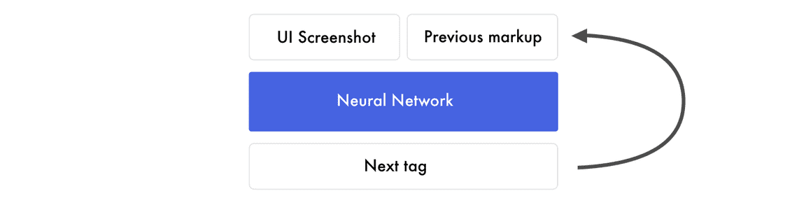
目前，自動化前端開發的最大阻礙是計算能力。但我們已經可以使用目前的深度學習算法，以及合成訓練數據來探索人工智能自動構建前端的方法。在本文中，作者將教神經網絡學習基於一張圖片和一個設計模板來編寫一個 HTML 和 CSS 網站。以下是該過程的簡要概述：

1）向訓練過的神經網絡輸入一個設計圖

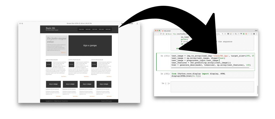
2）神經網絡將圖片轉化爲 HTML 標記語言

3）渲染輸出

我們將分三步從易到難構建三個不同的模型，首先，我們構建最簡單地版本來掌握移動部件。第二個版本 HTML 專注於自動化所有步驟，並簡要解釋神經網絡層。在最後一個版本 Bootstrap 中，我們將創建一個模型來思考和探索 LSTM 層。

代碼地址：

• https://github.com/emilwallner/Screenshot-to-code-in-Keras

• https://www.floydhub.com/emilwallner/projects/picturetocode

所有 FloydHub notebook 都在 floydhub 目錄中，本地 notebook 在 local 目錄中。

本文中的模型構建基於 Beltramelli 的論文《pix2code: Generating Code from a Graphical User Interface Screenshot》和 Jason Brownlee 的圖像描述生成教程，並使用 Python 和 Keras 完成。

核心邏輯

我們的目標是構建一個神經網絡，能夠生成與截圖對應的 HTML/CSS 標記語言。

訓練神經網絡時，你先提供幾個截圖和對應的 HTML 代碼。網絡通過逐個預測所有匹配的 HTML 標記語言來學習。預測下一個標記語言的標籤時，網絡接收到截圖和之前所有正確的標記。

這裏是一個簡單的訓練數據示例：https://docs.google.com/spreadsheets/d/1xXwarcQZAHluorveZsACtXRdmNFbwGtN3WMNhcTdEyQ/edit?usp=sharing。

創建逐詞預測的模型是現在最常用的方法，也是本教程使用的方法。

注意：每次預測時，神經網絡接收的是同樣的截圖。也就是說如果網絡需要預測 20 個單詞，它就會得到 20 次同樣的設計截圖。現在，不用管神經網絡的工作原理，只需要專注於神經網絡的輸入和輸出。

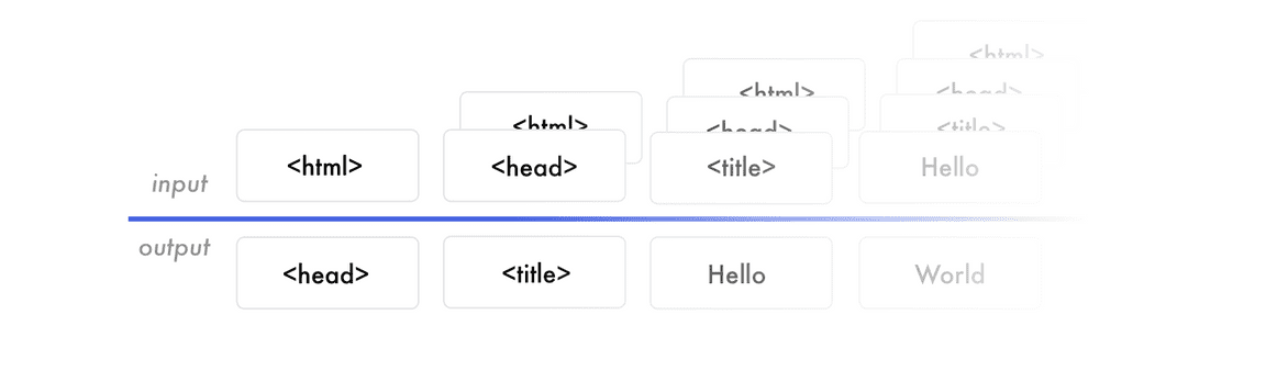
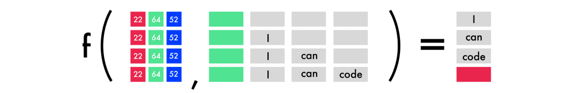
我們先來看前面的標記（markup）。假如我們訓練神經網絡的目的是預測句子「I can code」。當網絡接收「I」時，預測「can」。下一次時，網絡接收「I can」，預測「code」。它接收所有之前單詞，但只預測下一個單詞。

神經網絡根據數據創建特徵。神經網絡構建特徵以連接輸入數據和輸出數據。它必須創建表徵來理解每個截圖的內容和它所需要預測的 HTML 語法，這些都是爲預測下一個標記構建知識。把訓練好的模型應用到真實世界中和模型訓練過程差不多。

我們無需輸入正確的 HTML 標記，網絡會接收它目前生成的標記，然後預測下一個標記。預測從「起始標籤」（start tag）開始，到「結束標籤」（end tag）終止，或者達到最大限制時終止。

Hello World 版

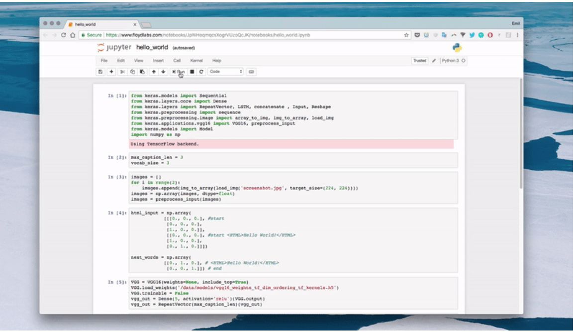
現在讓我們構建 Hello World 版實現。我們將饋送一張帶有「Hello World！」字樣的截屏到神經網絡中，並訓練它生成對應的標記語言。

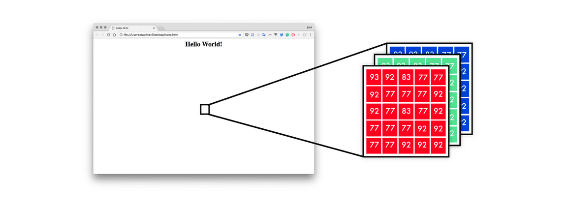
首先，神經網絡將原型設計轉換爲一組像素值。且每一個像素點有 RGB 三個通道，每個通道的值都在 0-255 之間。

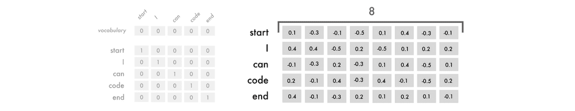
爲了以神經網絡能理解的方式表徵這些標記，我使用了 one-hot 編碼。因此句子「I can code」可以映射爲以下形式。

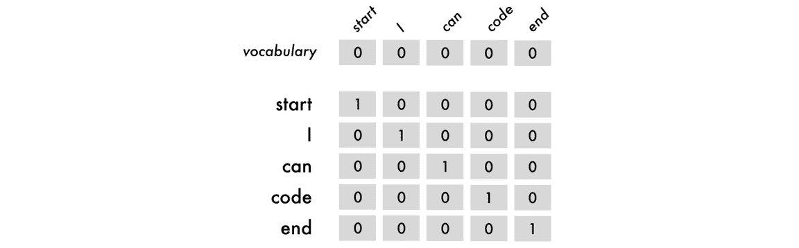
在上圖中，我們的編碼包含了開始和結束的標籤。這些標籤能爲神經網絡提供開始預測和結束預測的位置信息。以下是這些標籤的各種組合以及對應 one-hot 編碼的情況。

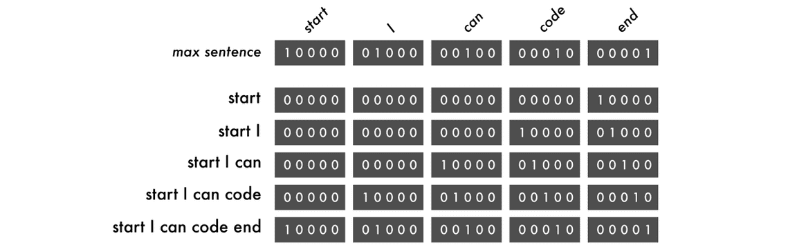
我們會使每個單詞在每一輪訓練中改變位置，因此這允許模型學習序列而不是記憶詞的位置。在下圖中有四個預測，每一行是一個預測。且左邊代表 RGB 三色通道和之前的詞，右邊代表預測結果和紅色的結束標籤。

1. #Length of longest sentence

2. max_caption_len = 3

3. #Size of vocabulary

4. vocab_size = 3

6. # Load one screenshot for each word and turn them into digits

7. images = []

8. fori inrange(2):

9. images.append(img_to_array(load_img('screenshot.jpg', target_size=(224, 224))))

10. images = np.array(images, dtype=float)

11. # Preprocess input for the VGG16 model

12. images = preprocess_input(images)

14. #Turn start tokens into one-hot encoding

15. html_input = np.array(

16. [[[0., 0., 0.], #start

17. [0., 0., 0.],

18. [1., 0., 0.]],

19. [[0., 0., 0.], #start Hello World!

20. [1., 0., 0.],

21. [0., 1., 0.]]])

23. #Turn next word into one-hot encoding

24. next_words = np.array(

25. [[0., 1., 0.], # Hello World!

26. [0., 0., 1.]]) # end

28. # Load the VGG16 model trained on imagenet and output the classification feature

29. VGG = VGG16(weights='imagenet', include_top=True)

30. # Extract the features from the image

31. features = VGG.predict(images)

33. #Load the feature to the network, apply a dense layer, and repeat the vector

34. vgg_feature = Input(shape=(1000,))

35. vgg_feature_dense = Dense(5)(vgg_feature)

36. vgg_feature_repeat = RepeatVector(max_caption_len)(vgg_feature_dense)

37. # Extract information from the input seqence

38. language_input = Input(shape=(vocab_size, vocab_size))

39. language_model = LSTM(5, return_sequences=True)(language_input)

41. # Concatenate the information from the image and the input

42. decoder = concatenate([vgg_feature_repeat, language_model])

43. # Extract information from the concatenated output

44. decoder = LSTM(5, return_sequences=False)(decoder)

45. # Predict which word comes next

46. decoder_output = Dense(vocab_size, activation='softmax')(decoder)

47. # Compile and run the neural network

48. model = Model(inputs=[vgg_feature, language_input], outputs=decoder_output)

49. model.compile(loss='categorical_crossentropy', optimizer='rmsprop')

51. # Train the neural network

52. model.fit([features, html_input], next_words, batch_size=2, shuffle=False, epochs=1000)

在 Hello World 版本中，我們使用三個符號「start」、「Hello World」和「end」。字符級的模型要求更小的詞彙表和受限的神經網絡，而單詞級的符號在這裏可能有更好的性能。

以下是執行預測的代碼：

1. # Create an empty sentence and insert the start token

2. sentence = np.zeros((1, 3, 3)) # [[0,0,0], [0,0,0], [0,0,0]]

3. start_token = [1., 0., 0.] # start

4. sentence[0][2] = start_token # place start in empty sentence

6. # Making the first prediction with the start token

7. second_word = model.predict([np.array([features[1]]), sentence])

9. # Put the second word in the sentence and make the final prediction

10. sentence[0][1] = start_token

11. sentence[0][2] = np.round(second_word)

12. third_word = model.predict([np.array([features[1]]), sentence])

14. # Place the start token and our two predictions in the sentence

15. sentence[0][0] = start_token

16. sentence[0][1] = np.round(second_word)

17. sentence[0][2] = np.round(third_word)

19. # Transform our one-hot predictions into the final tokens

20. vocabulary = ["start", "

    Hello World!

    ", "end"]

21. fori insentence[0]:

22. print(vocabulary[np.argmax(i)], end=' ')

輸出

• 10 epochs: start start start

• 100 epochs: start

  Hello World!

  Hello World!

• 300 epochs: start

  Hello World!

  end

我走過的坑：

• 在收集數據之前構建第一個版本。在本項目的早期階段，我設法獲得 Geocities 託管網站的舊版存檔，它有 3800 萬的網站。但我忽略了減少 100K 大小詞彙所需要的巨大工作量。

• 訓練一個 TB 級的數據需要優秀的硬件或極其有耐心。在我的 Mac 遇到幾個問題後，最終用上了強大的遠程服務器。我預計租用 8 個現代 CPU 和 1 GPS 內部鏈接以運行我的工作流。

• 在理解輸入與輸出數據之前，其它部分都似懂非懂。輸入 X 是屏幕的截圖和以前標記的標籤，輸出 Y 是下一個標記的標籤。當我理解這一點時，其它問題都更加容易弄清了。此外，嘗試其它不同的架構也將更加容易。

• 圖片到代碼的網絡其實就是自動描述圖像的模型。即使我意識到了這一點，但仍然錯過了很多自動圖像摘要方面的論文，因爲它們看起來不夠炫酷。一旦我意識到了這一點，我對問題空間的理解就變得更加深刻了。

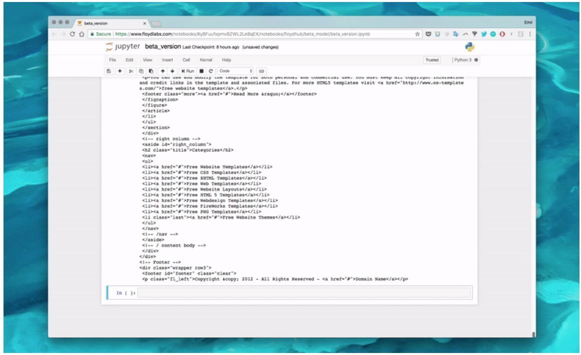
在 FloydHub 上運行代碼

FloydHub 是一個深度學習訓練平臺，我自從開始學習深度學習時就對它有所瞭解，我也常用它訓練和管理深度學習試驗。我們能安裝它並在 10 分鐘內運行第一個模型，它是在雲 GPU 上訓練模型最好的選擇。若果讀者沒用過 FloydHub，可以花 10 分鐘左右安裝並瞭解。

FloydHub 地址：https://www.floydhub.com/

複製 Repo：

1. https://github.com/emilwallner/Screenshot-to-code-in-Keras.git

登錄並初始化 FloydHub 命令行工具：

1. cd Screenshot-to-code-in-Keras

2. floyd login

3. floyd init s2c

在 FloydHub 雲 GPU 機器上運行 Jupyter notebook：

1. floyd run --gpu --env tensorflow-1.4--data emilwallner/datasets/imagetocode/2:data --mode jupyter

所有的 notebook 都放在 floydbub 目錄下。一旦我們開始運行模型，那麼在 floydhub/Helloworld/helloworld.ipynb 下可以找到第一個 Notebook。更多詳情請查看本項目早期的 flags。

HTML 版本

在這個版本中，我們將關注與創建一個可擴展的神經網絡模型。該版本並不能直接從隨機網頁預測 HTML，但它是探索動態問題不可缺少的步驟。

概覽

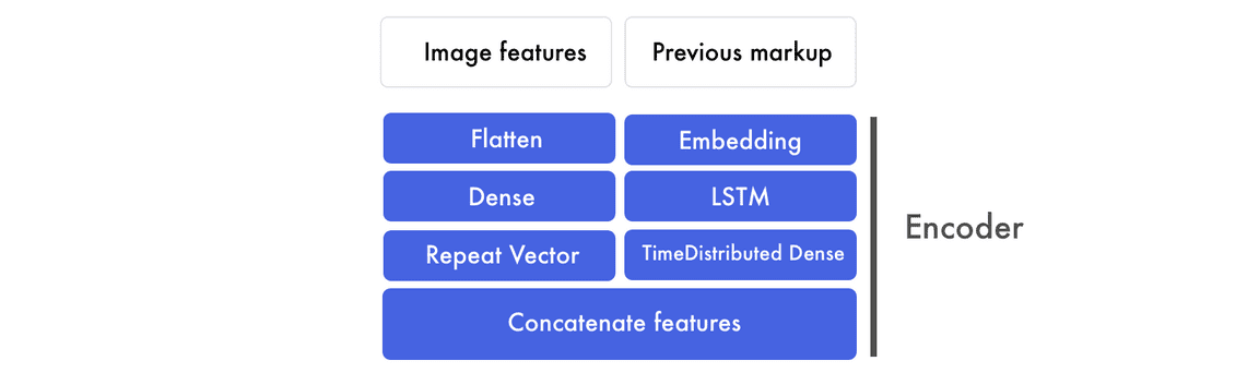
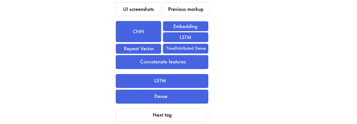
如果我們將前面的架構擴展爲以下右圖展示的結構，那麼它就能更高效地處理識別與轉換過程。

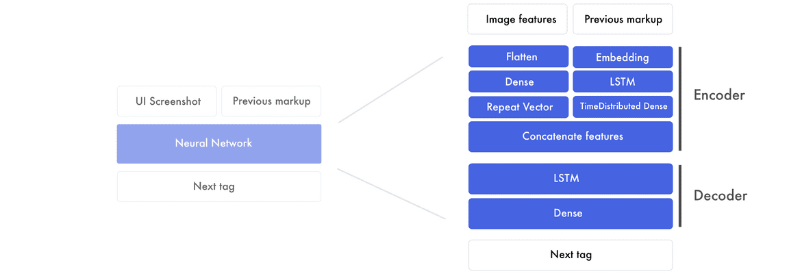
該架構主要有兩個部，即編碼器與解碼器。編碼器是我們創建圖像特徵和前面標記特徵（markup features）的部分。特徵是網絡創建原型設計和標記語言之間聯繫的構建塊。在編碼器的末尾，我們將圖像特徵傳遞給前面標記的每一個單詞。隨後解碼器將結合原型設計特徵和標記特徵以創建下一個標籤的特徵，這一個特徵可以通過全連接層預測下一個標籤。

設計原型的特徵

因爲我們需要爲每個單詞插入一個截屏，這將會成爲訓練神經網絡的瓶頸。因此我們抽取生成標記語言所需要的信息來替代直接使用圖像。這些抽取的信息將通過預訓練的 CNN 編碼到圖像特徵中，且我們將使用分類層之前的層級輸出以抽取特徵。

我們最終得到 1536 個 8*8 的特徵圖，雖然我們很難直觀地理解它，但神經網絡能夠從這些特徵中抽取元素的對象和位置。

標記特徵

在 Hello World 版本中，我們使用 one-hot 編碼以表徵標記。而在該版本中，我們將使用詞嵌入表徵輸入並使用 one-hot 編碼表示輸出。我們構建每個句子的方式保持不變，但我們映射每個符號的方式將會變化。one-hot 編碼將每一個詞視爲獨立的單元，而詞嵌入會將輸入數據表徵爲一個實數列表，這些實數表示標記標籤之間的關係。

上面詞嵌入的維度爲 8，但一般詞嵌入的維度會根據詞彙表的大小在 50 到 500 間變動。以上每個單詞的八個數值就類似於神經網絡中的權重，它們傾向於刻畫單詞之間的聯繫（Mikolov alt el., 2013）。這就是我們開始部署標記特徵（markup features）的方式，而這些神經網絡訓練的特徵會將輸入數據和輸出數據聯繫起來。

編碼器

我們現在將詞嵌入饋送到 LSTM 中，並期望能返回一系列的標記特徵。這些標記特徵隨後會饋送到一個 Time Distributed 密集層，該層級可以視爲有多個輸入和輸出的全連接層。

和嵌入與 LSTM 層相平行的還有另外一個處理過程，其中圖像特徵首先會展開成一個向量，然後再饋送到一個全連接層而抽取出高級特徵。這些圖像特徵隨後會與標記特徵相級聯而作爲編碼器的輸出。

標記特徵

如下圖所示，現在我們將詞嵌入投入到 LSTM 層中，所有的語句都會用零填充以獲得相同的向量長度。

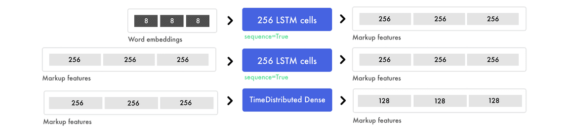
爲了混合信號並尋找高級模式，我們運用了一個 TimeDistributed 密集層以抽取標記特徵。TimeDistributed 密集層和一般的全連接層非常相似，且它有多個輸入與輸出。

圖像特徵

對於另一個平行的過程，我們需要將圖像的所有像素值展開成一個向量，因此信息不會被改變，它們只會用來識別。

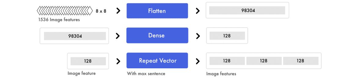
如上，我們會通過全連接層混合信號並抽取更高級的概念。因爲我們並不只是處理一個輸入值，因此使用一般的全連接層就行了。

級聯圖像特徵和標記特徵

所有的語句都被填充以創建三個標記特徵。因爲我們已經預處理了圖像特徵，所以我們能爲每一個標記特徵添加圖像特徵。

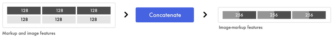
如上，在複製圖像特徵到對應的標記特徵後，我們得到了新的圖像-標記特徵（image-markup features），這就是我們饋送到解碼器的輸入值。

解碼器

現在，我們使用圖像-標記特徵來預測下一個標籤。

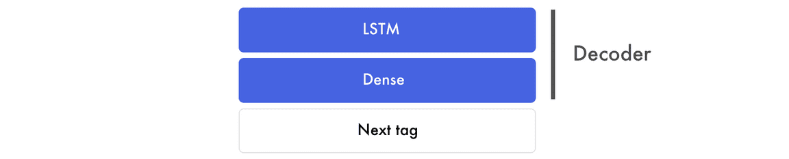
在下面的案例中，我們使用三個圖像-標籤特徵對來輸出下一個標籤特徵。注意 LSTM 層不應該返回一個長度等於輸入序列的向量，而只需要預測預測一個特徵。在我們的案例中，這個特徵將預測下一個標籤，它包含了最後預測的信息。

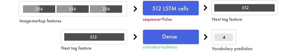
最後的預測

密集層會像傳統前饋網絡那樣工作，它將下一個標籤特徵中的 512 個值與最後的四個預測連接起來，即我們在詞彙表所擁有的四個單詞：start、hello、world 和 end。密集層最後採用的 softmax 函數會爲四個類別產生一個概率分佈，例如 [0.1, 0.1, 0.1, 0.7] 將預測第四個詞爲下一個標籤。

1. # Load the images and preprocess them for inception-resnet

2. images = []

3. all_filenames = listdir('images/')

4. all_filenames.sort()

5. forfilename inall_filenames:

6. images.append(img_to_array(load_img('images/'+filename, target_size=(299, 299))))

7. images = np.array(images, dtype=float)

8. images = preprocess_input(images)

10. # Run the images through inception-resnet and extract the features without the classification layer

11. IR2 = InceptionResNetV2(weights='imagenet', include_top=False)

12. features = IR2.predict(images)

15. # We will cap each input sequence to 100 tokens

16. max_caption_len = 100

17. # Initialize the function that will create our vocabulary

18. tokenizer = Tokenizer(filters='', split=" ", lower=False)

20. # Read a document and return a string

21. defload_doc(filename):

22. file = open(filename, 'r')

23. text = file.read()

24. file.close()

25. returntext

27. # Load all the HTML files

28. X = []

29. all_filenames = listdir('html/')

30. all_filenames.sort()

31. forfilename inall_filenames:

32. X.append(load_doc('html/'+filename))

34. # Create the vocabulary from the html files

35. tokenizer.fit_on_texts(X)

37. # Add +1 to leave space for empty words

38. vocab_size = len(tokenizer.word_index) + 1

39. # Translate each word in text file to the matching vocabulary index

40. sequences = tokenizer.texts_to_sequences(X)

41. # The longest HTML file

42. max_length = max(len(s) fors insequences)

44. # Intialize our final input to the model

45. X, y, image_data = list(), list(), list()

46. forimg_no, seq inenumerate(sequences):

47. fori inrange(1, len(seq)):

48. # Add the entire sequence to the input and only keep the next word for the output

49. in_seq, out_seq = seq[:i], seq[i]

50. # If the sentence is shorter than max_length, fill it up with empty words

51. in_seq = pad_sequences([in_seq], maxlen=max_length)[0]

52. # Map the output to one-hot encoding

53. out_seq = to_categorical([out_seq], num_classes=vocab_size)[0]

54. # Add and image corresponding to the HTML file

55. image_data.append(features[img_no])

56. # Cut the input sentence to 100 tokens, and add it to the input data

57. X.append(in_seq[-100:])

58. y.append(out_seq)

60. X, y, image_data = np.array(X), np.array(y), np.array(image_data)

62. # Create the encoder

63. image_features = Input(shape=(8, 8, 1536,))

64. image_flat = Flatten()(image_features)

65. image_flat = Dense(128, activation='relu')(image_flat)

66. ir2_out = RepeatVector(max_caption_len)(image_flat)

68. language_input = Input(shape=(max_caption_len,))

69. language_model = Embedding(vocab_size, 200, input_length=max_caption_len)(language_input)

70. language_model = LSTM(256, return_sequences=True)(language_model)

71. language_model = LSTM(256, return_sequences=True)(language_model)

72. language_model = TimeDistributed(Dense(128, activation='relu'))(language_model)

74. # Create the decoder

75. decoder = concatenate([ir2_out, language_model])

76. decoder = LSTM(512, return_sequences=False)(decoder)

77. decoder_output = Dense(vocab_size, activation='softmax')(decoder)

79. # Compile the model

80. model = Model(inputs=[image_features, language_input], outputs=decoder_output)

81. model.compile(loss='categorical_crossentropy', optimizer='rmsprop')

83. # Train the neural network

84. model.fit([image_data, X], y, batch_size=64, shuffle=False, epochs=2)

86. # map an integer to a word

87. defword_for_id(integer, tokenizer):

88. forword, index intokenizer.word_index.items():

89. ifindex == integer:

90. returnword

91. returnNone

93. # generate a deion for an image

94. defgenerate_desc(model, tokenizer, photo, max_length):

95. # seed the generation process

96. in_text = 'START'

97. # iterate over the whole length of the sequence

98. fori inrange(900):

99. # integer encode input sequence

100. sequence = tokenizer.texts_to_sequences([in_text])[0][-100:]

101. # pad input

102. sequence = pad_sequences([sequence], maxlen=max_length)

103. # predict next word

104. yhat = model.predict([photo,sequence], verbose=0)

105. # convert probability to integer

106. yhat = np.argmax(yhat)

107. # map integer to word

108. word = word_for_id(yhat, tokenizer)

109. # stop if we cannot map the word

110. ifword isNone:

111. break

112. # append as input for generating the next word

113. in_text += ' '+ word

114. # Print the prediction

115. print(' '+ word, end='')

116. # stop if we predict the end of the sequence

117. ifword == 'END':

118. break

119. return

121. # Load and image, preprocess it for IR2, extract features and generate the HTML

122. test_image = img_to_array(load_img('images/87.jpg', target_size=(299, 299)))

123. test_image = np.array(test_image, dtype=float)

124. test_image = preprocess_input(test_image)

125. test_features = IR2.predict(np.array([test_image]))

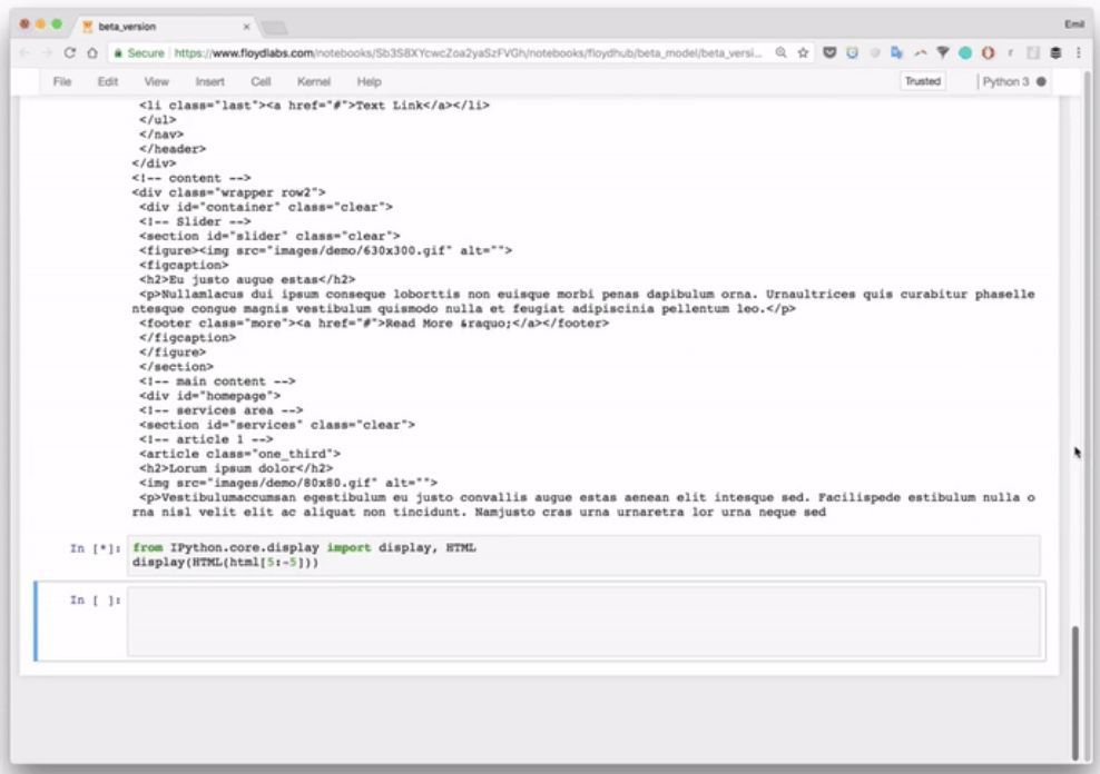
126. generate_desc(model, tokenizer, np.array(test_features), 100)

輸出

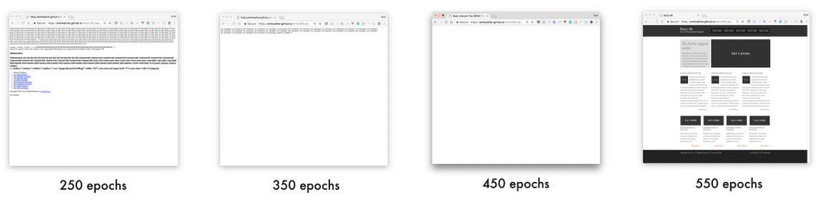
訓練不同輪數所生成網站的地址：

• 250 epochs：https://emilwallner.github.io/html/250_epochs/

• 350 epochs：https://emilwallner.github.io/html/350_epochs/

• 450 epochs：https://emilwallner.github.io/html/450_epochs/

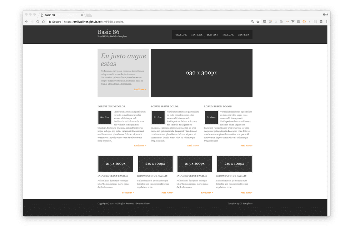
• 550 epochs：https://emilwallner.github.io/html/550_epochs/

我走過的坑：

• 我認爲理解 LSTM 比 CNN 要難一些。當我展開 LSTM 後，它們會變得容易理解一些。此外，我們在嘗試理解 LSTM 前，可以先關注輸入與輸出特徵。

• 從頭構建一個詞彙表要比壓縮一個巨大的詞彙表容易得多。這樣的構建包括字體、div 標籤大小、變量名的 hex 顏色和一般單詞。

• 大多數庫是爲解析文本文檔而構建。在庫的使用文檔中，它們會告訴我們如何通過空格進行分割，而不是代碼，我們需要自定義解析的方式。

• 我們可以從 ImageNet 上預訓練的模型抽取特徵。然而，相對於從頭訓練的 pix2code 模型，損失要高 30% 左右。此外，我對於使用基於網頁截屏預訓練的 inception-resnet 網絡很有興趣。

Bootstrap 版本

在最終版本中，我們使用 pix2code 論文中生成 bootstrap 網站的數據集。使用 Twitter 的 Bootstrap 庫（https://getbootstrap.com/），我們可以結合 HTML 和 CSS，降低詞彙表規模。

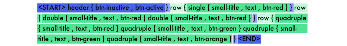
我們將使用這一版本爲之前未見過的截圖生成標記。我們還深入研究它如何構建截圖和標記的先驗知識。

我們不在 bootstrap 標記上訓練，而是使用 17 個簡化 token，將其編譯成 HTML 和 CSS。數據集（https://github.com/tonybeltramelli/pix2code/tree/master/datasets）包括 1500 個測試截圖和 250 個驗證截圖。平均每個截圖有 65 個 token，一共有 96925 個訓練樣本。

我們稍微修改一下 pix2code 論文中的模型，使之預測網絡組件的準確率達到 97%。

端到端方法

從預訓練模型中提取特徵在圖像描述生成模型中效果很好。但是幾次實驗後，我發現 pix2code 的端到端方法效果更好。在我們的模型中，我們用輕量級卷積神經網絡替換預訓練圖像特徵。我們不使用最大池化來增加信息密度，而是增加步幅。這可以保持前端元素的位置和顏色。

存在兩個核心模型：卷積神經網絡（CNN）和循環神經網絡（RNN）。最常用的循環神經網絡是長短期記憶（LSTM）網絡。我之前的文章中介紹過 CNN 教程，本文主要介紹 LSTM。

理解 LSTM 中的時間步

關於 LSTM 比較難理解的是時間步。我們的原始神經網絡有兩個時間步，如果你給它「Hello」，它就會預測「World」。但是它會試圖預測更多時間步。下例中，輸入有四個時間步，每個單詞對應一個時間步。

LSTM 適合時序數據的輸入，它是一種適合順序信息的神經網絡。模型展開圖示如下，對於每個循環步，你需要保持同樣的權重。

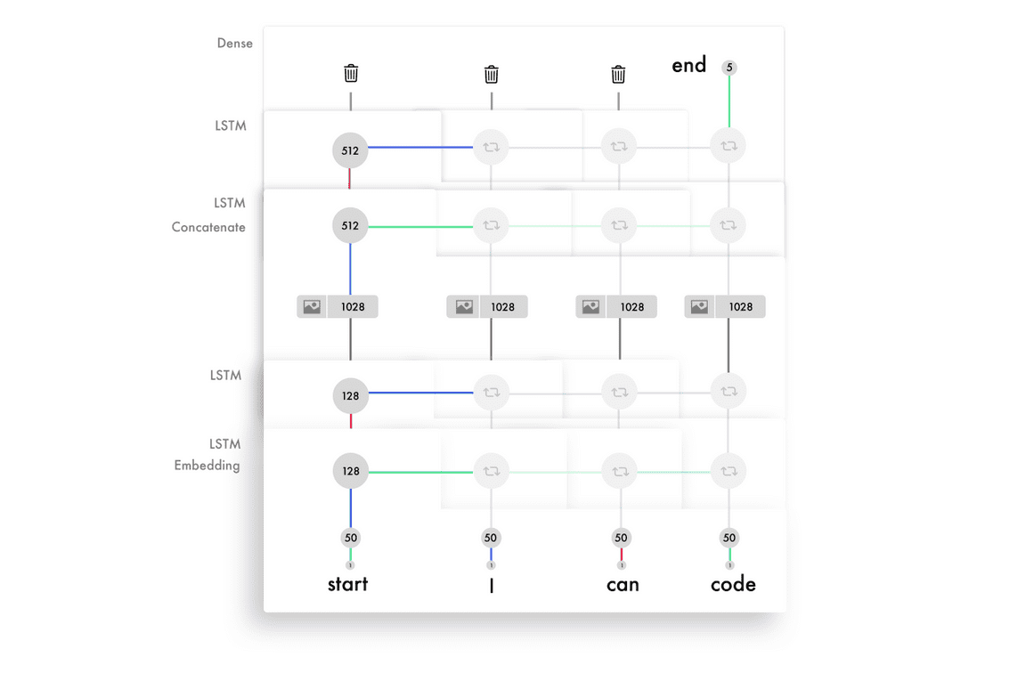
加權後的輸入與輸出特徵在級聯後輸入到激活函數，並作爲當前時間步的輸出。因爲我們重複利用了相同的權重，它們將從一些輸入獲取信息並構建序列的知識。下面是 LSTM 在每一個時間步上的簡化版處理過程：

理解 LSTM 層級中的單元

每一層 LSTM 單元的總數決定了它記憶的能力，同樣也對應於每一個輸出特徵的維度大小。LSTM 層級中的每一個單元將學習如何追蹤句法的不同方面。以下是一個 LSTM 單元追蹤標籤行信息的可視化，它是我們用來訓練 bootstrap 模型的簡單標記語言。

每一個 LSTM 單元會維持一個單元狀態，我們可以將單元狀態視爲記憶。權重和激活值可使用不同的方式修正狀態值，這令 LSTM 層可以通過保留或遺忘輸入信息而得到精調。除了處理當前輸入信息與輸出信息，LSTM 單元還需要修正記憶狀態以傳遞到下一個時間步。

1. dir_name = 'resources/eval_light/'

3. # Read a file and return a string

4. defload_doc(filename):

5. file = open(filename, 'r')

6. text = file.read()

7. file.close()

8. returntext

10. defload_data(data_dir):

11. text = []

12. images = []

13. # Load all the files and order them

14. all_filenames = listdir(data_dir)

15. all_filenames.sort()

16. forfilename in(all_filenames):

17. iffilename[-3:] == "npz":

18. # Load the images already prepared in arrays

19. image = np.load(data_dir+filename)

20. images.append(image['features'])

21. else:

22. # Load the boostrap tokens and rap them in a start and end tag

23. syntax = ' ' + load_doc(data_dir+filename) + ' '

24. # Seperate all the words with a single space

25. syntax = ' '.join(syntax.split())

26. # Add a space after each comma

27. syntax = syntax.replace(',', ' ,')

28. text.append(syntax)

29. images = np.array(images, dtype=float)

30. returnimages, text

32. train_features, texts = load_data(dir_name)

34. # Initialize the function to create the vocabulary

35. tokenizer = Tokenizer(filters='', split=" ", lower=False)

36. # Create the vocabulary

37. tokenizer.fit_on_texts([load_doc('bootstrap.vocab')])

39. # Add one spot for the empty word in the vocabulary

40. vocab_size = len(tokenizer.word_index) + 1

41. # Map the input sentences into the vocabulary indexes

42. train_sequences = tokenizer.texts_to_sequences(texts)

43. # The longest set of boostrap tokens

44. max_sequence = max(len(s) fors intrain_sequences)

45. # Specify how many tokens to have in each input sentence

46. max_length = 48

48. defpreprocess_data(sequences, features):

49. X, y, image_data = list(), list(), list()

50. forimg_no, seq inenumerate(sequences):

51. fori inrange(1, len(seq)):

52. # Add the sentence until the current count(i) and add the current count to the output

53. in_seq, out_seq = seq[:i], seq[i]

54. # Pad all the input token sentences to max_sequence

55. in_seq = pad_sequences([in_seq], maxlen=max_sequence)[0]

56. # Turn the output into one-hot encoding

57. out_seq = to_categorical([out_seq], num_classes=vocab_size)[0]

58. # Add the corresponding image to the boostrap token file

59. image_data.append(features[img_no])

60. # Cap the input sentence to 48 tokens and add it

61. X.append(in_seq[-48:])

62. y.append(out_seq)

63. returnnp.array(X), np.array(y), np.array(image_data)

65. X, y, image_data = preprocess_data(train_sequences, train_features)

67. #Create the encoder

68. image_model = Sequential()

69. image_model.add(Conv2D(16, (3, 3), padding='valid', activation='relu', input_shape=(256, 256, 3,)))

70. image_model.add(Conv2D(16, (3,3), activation='relu', padding='same', strides=2))

71. image_model.add(Conv2D(32, (3,3), activation='relu', padding='same'))

72. image_model.add(Conv2D(32, (3,3), activation='relu', padding='same', strides=2))

73. image_model.add(Conv2D(64, (3,3), activation='relu', padding='same'))

74. image_model.add(Conv2D(64, (3,3), activation='relu', padding='same', strides=2))

75. image_model.add(Conv2D(128, (3,3), activation='relu', padding='same'))

77. image_model.add(Flatten())

78. image_model.add(Dense(1024, activation='relu'))

79. image_model.add(Dropout(0.3))

80. image_model.add(Dense(1024, activation='relu'))

81. image_model.add(Dropout(0.3))

83. image_model.add(RepeatVector(max_length))

85. visual_input = Input(shape=(256, 256, 3,))

86. encoded_image = image_model(visual_input)

88. language_input = Input(shape=(max_length,))

89. language_model = Embedding(vocab_size, 50, input_length=max_length, mask_zero=True)(language_input)

90. language_model = LSTM(128, return_sequences=True)(language_model)

91. language_model = LSTM(128, return_sequences=True)(language_model)

93. #Create the decoder

94. decoder = concatenate([encoded_image, language_model])

95. decoder = LSTM(512, return_sequences=True)(decoder)

96. decoder = LSTM(512, return_sequences=False)(decoder)

97. decoder = Dense(vocab_size, activation='softmax')(decoder)

99. # Compile the model

100. model = Model(inputs=[visual_input, language_input], outputs=decoder)

101. optimizer = RMSprop(lr=0.0001, clipvalue=1.0)

102. model.compile(loss='categorical_crossentropy', optimizer=optimizer)

104. #Save the model for every 2nd epoch

105. filepath="org-weights-epoch-{epoch:04d}--val_loss-{val_loss:.4f}--loss-{loss:.4f}.hdf5"

106. checkpoint = ModelCheckpoint(filepath, monitor='val_loss', verbose=1, save_weights_only=True, period=2)

107. callbacks_list = [checkpoint]

109. # Train the model

110. model.fit([image_data, X], y, batch_size=64, shuffle=False, validation_split=0.1, callbacks=callbacks_list, verbose=1, epochs=50)

測試準確率

找到一種測量準確率的優秀方法非常棘手。比如一個詞一個詞地對比，如果你的預測中有一個詞不對照，準確率可能就是 0。如果你把百分百對照的單詞移除一個，最終的準確率可能是 99/100。

我使用的是 BLEU 分值，它在機器翻譯和圖像描述模型實踐上都是最好的。它把句子分解成 4 個 n-gram，從 1-4 個單詞的序列。在下面的預測中，「cat」應該是「code」。

爲了得到最終的分值，每個的分值需要乘以 25%，(4/5) × 0.25 + (2/4) × 0.25 + (1/3) ×0.25 + (0/2) ×0.25 = 0.2 + 0.125 + 0.083 + 0 = 0.408。然後用總和乘以句子長度的懲罰函數。因爲在我們的示例中，長度是正確的，所以它就直接是我們的最終得分。

你可以增加 n-gram 的數量，4 個 n-gram 的模型是最爲對應人類翻譯的。我建議你閱讀下面的代碼：

1. #Create a function to read a file and return its content

2. defload_doc(filename):

3. file = open(filename, 'r')

4. text = file.read()

5. file.close()

6. returntext

8. defload_data(data_dir):

9. text = []

10. images = []

11. files_in_folder = os.listdir(data_dir)

12. files_in_folder.sort()

13. forfilename intqdm(files_in_folder):

14. #Add an image

15. iffilename[-3:] == "npz":

16. image = np.load(data_dir+filename)

17. images.append(image['features'])

18. else:

19. # Add text and wrap it in a start and end tag

20. syntax = ' ' + load_doc(data_dir+filename) + ' '

21. #Seperate each word with a space

22. syntax = ' '.join(syntax.split())

23. #Add a space between each comma

24. syntax = syntax.replace(',', ' ,')

25. text.append(syntax)

26. images = np.array(images, dtype=float)

27. returnimages, text

29. #Intialize the function to create the vocabulary

30. tokenizer = Tokenizer(filters='', split=" ", lower=False)

31. #Create the vocabulary in a specific order

32. tokenizer.fit_on_texts([load_doc('bootstrap.vocab')])

34. dir_name = '../../../../eval/'

35. train_features, texts = load_data(dir_name)

37. #load model and weights

38. json_file = open('../../../../model.json', 'r')

39. loaded_model_json = json_file.read()

40. json_file.close()

41. loaded_model = model_from_json(loaded_model_json)

42. # load weights into new model

43. loaded_model.load_weights("../../../../weights.hdf5")

44. print("Loaded model from disk")

46. # map an integer to a word

47. defword_for_id(integer, tokenizer):

48. forword, index intokenizer.word_index.items():

49. ifindex == integer:

50. returnword

51. returnNone

52. print(word_for_id(17, tokenizer))

54. # generate a deion for an image

55. defgenerate_desc(model, tokenizer, photo, max_length):

56. photo = np.array([photo])

57. # seed the generation process

58. in_text = ' '

59. # iterate over the whole length of the sequence

60. print('nPrediction---->nn ' , end='')

61. fori inrange(150):

62. # integer encode input sequence

63. sequence = tokenizer.texts_to_sequences([in_text])[0]

64. # pad input

65. sequence = pad_sequences([sequence], maxlen=max_length)

66. # predict next word

67. yhat = loaded_model.predict([photo, sequence], verbose=0)

68. # convert probability to integer

69. yhat = argmax(yhat)

70. # map integer to word

71. word = word_for_id(yhat, tokenizer)

72. # stop if we cannot map the word

73. ifword isNone:

74. break

75. # append as input for generating the next word

76. in_text += word + ' '

77. # stop if we predict the end of the sequence

78. print(word + ' ', end='')

79. ifword == ' ' :

80. break

81. returnin_text

84. max_length = 48

86. # evaluate the skill of the model

87. defevaluate_model(model, deions, photos, tokenizer, max_length):

88. actual, predicted = list(), list()

89. # step over the whole set

90. fori inrange(len(texts)):

91. yhat = generate_desc(model, tokenizer, photos[i], max_length)

92. # store actual and predicted

93. print('nnReal---->nn'+ texts[i])

94. actual.append([texts[i].split()])

95. predicted.append(yhat.split())

96. # calculate BLEU score

97. bleu = corpus_bleu(actual, predicted)

98. returnbleu, actual, predicted

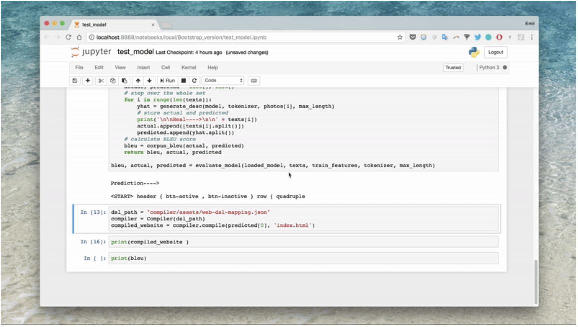
100. bleu, actual, predicted = evaluate_model(loaded_model, texts, train_features, tokenizer, max_length)

102. #Compile the tokens into HTML and css

103. dsl_path = "compiler/assets/web-dsl-mapping.json"

104. compiler = Compiler(dsl_path)

105. compiled_website = compiler.compile(predicted[0], 'index.html')

107. print(compiled_website )

108. print(bleu)

輸出

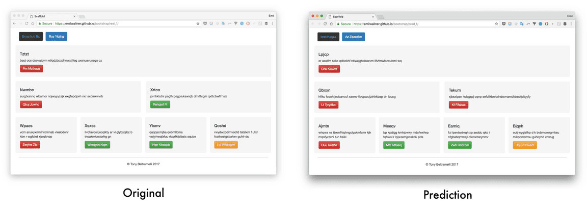
樣本輸出的鏈接：

• Generated website 1 - Original 1 (https://emilwallner.github.io/bootstrap/real_1/)

• Generated website 2 - Original 2 (https://emilwallner.github.io/bootstrap/real_2/)

• Generated website 3 - Original 3 (https://emilwallner.github.io/bootstrap/real_3/)

• Generated website 4 - Original 4 (https://emilwallner.github.io/bootstrap/real_4/)

• Generated website 5 - Original 5 (https://emilwallner.github.io/bootstrap/real_5/)

我走過的坑：

• 理解模型的弱點而不是測試隨機模型。首先我使用隨機的東西，比如批歸一化、雙向網絡，並嘗試實現注意力機制。在查看測試數據，並知道其無法高精度地預測顏色和位置之後，我意識到 CNN 存在一個弱點。這致使我使用增加的步幅來取代最大池化。驗證損失從 0.12 降至 0.02，BLEU 分值從 85% 增加至 97%。

• 如果它們相關，則只使用預訓練模型。在小數據的情況下，我認爲一個預訓練圖像模型將會提升性能。從我的實驗來看，端到端模型訓練更慢，需要更多內存，但是精確度會提升 30%。

• 當你在遠程服務器上運行模型，我們需要爲一些不同做好準備。在我的 mac 上，它按照字母表順序讀取文檔。但是在服務器上，它被隨機定位。這在代碼和截圖之間造成了不匹配。

下一步

前端開發是深度學習應用的理想空間。數據容易生成，並且當前深度學習算法可以映射絕大部分邏輯。一個最讓人激動的領域是注意力機制在 LSTM 上的應用。這不僅會提升精確度，還可以使我們可視化 CNN 在生成標記時所聚焦的地方。注意力同樣是標記、可定義模板、腳本和最終端之間通信的關鍵。注意力層要追蹤變量，使網絡可以在編程語言之間保持通信。

但是在不久的將來，最大的影響將會來自合成數據的可擴展方法。接着你可以一步步添加字體、顏色和動畫。目前爲止，大多數進步發生在草圖（sketches）方面並將其轉化爲模版應用。在不到兩年的時間裏，我們將創建一個草圖，它會在一秒之內找到相應的前端。Airbnb 設計團隊與 Uizard 已經創建了兩個正在使用的原型。下面是一些可能的試驗過程：

實驗

開始

• 運行所有模型

• 嘗試不同的超參數

• 測試一個不同的 CNN 架構

• 添加雙向 LSTM 模型

• 用不同數據集實現模型

進一步實驗

• 使用相應的語法創建一個穩定的隨機應用/網頁生成器

• 從草圖到應用模型的數據。自動將應用/網頁截圖轉化爲草圖，並使用 GAN 創建多樣性。

• 應用注意力層可視化每一預測的圖像聚焦，類似於這個模型

• 爲模塊化方法創建一個框架。比如，有字體的編碼器模型，一個用於顏色，另一個用於排版，並使用一個解碼器整合它們。穩定的圖像特徵是一個好的開始。

• 饋送簡單的 HTML 組件到神經網絡中，並使用 CSS 教其生成動畫。使用注意力方法並可視化兩個輸入源的聚焦將會很迷人。

原文鏈接：https://blog.floydhub.com/turning-design-mockups-into-code-with-deep-learning/